There are many sophisticated tools dedicated to Monte Carlo simulation, but Excel is powerful enough to handle a variety of simulation needs. Here are the basic steps of simulation in Excel. First the users build a decision model in a spreadsheet and specify what are the sources of uncertainty. Excel can then generate random numbers from those uncertainties representing possible outcome scenarios. Then this can be repeated many many times, hundreds, thousands or even more if necessary. Lastly summary statistics are computed, so that we can get a good sense of what we should expect when those uncertainties unfold.
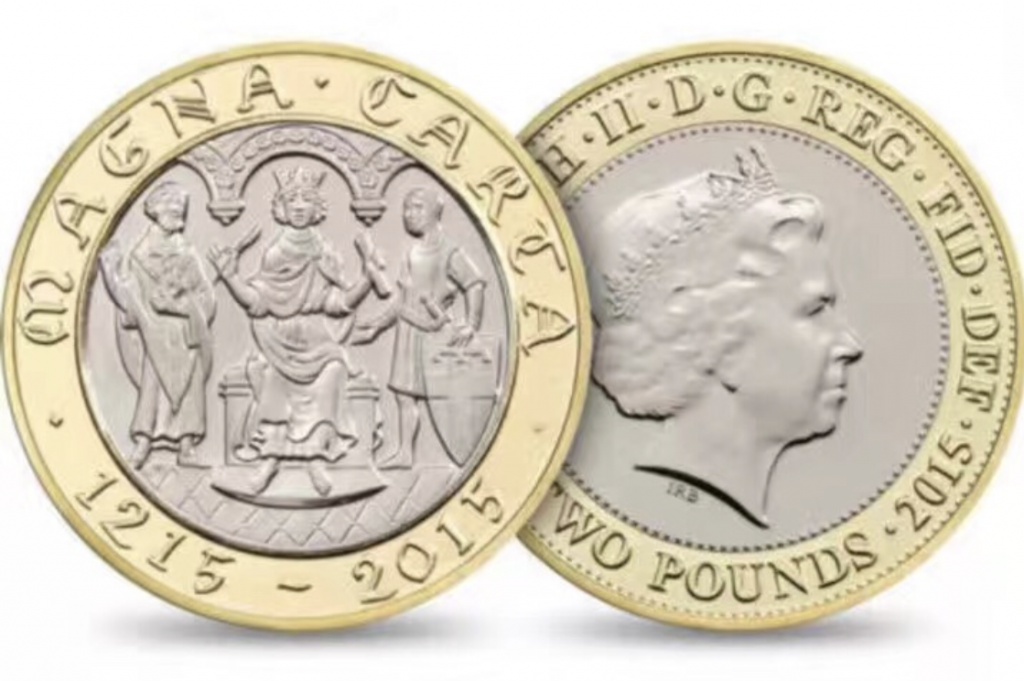
Now let us turn to what is perhaps the simplest of all simulations: a coin toss. It is the simplest because it has the simplest outcome: head, or tail. Or equivalently, we can say the outcome is binary: 0, or 1. Statistically, it is called the Bernoulli distribution, named after Swiss mathematician Jacob Bernoulli. where the probability of getting a head is 50% for a fair coin.
The key here is Excel’s RAND function. It simulates a random uniform [0,1] distribution. In other words, it draws a random number that is between 0 and 1.
It turns out that the cumulative distribution functions (CDF) of any statistical random distribution, whether discrete or continuous, are all distributed this way.
In the case of a coin toss, we can just say if the CDF is less than 0.5, it is a head, and if it is great than 0.5, then it is a tail. That is how you map a CDF into an outcome.
But if the above confused you, don’t worry. The video below shows how to do that in Excel.
You can download the Excel file here.
